RESOURCES
For many years now, we’ve been sharing useful resources and media stories related to our research projects. As a leading Science Laboratory in the San Francisco area, it’s important for us to engage with the community and keep them informed about the incredible work and developments they’re helping to support.


Decoding conditions from phase data
Decoding (classifying) experimental conditions from neural oscillatory phase
One way to estimate how well a neural signal represents a specific experimental condition among multiple other experimental conditions is to use a single-trial classification approach. Several powerful classification algorithms are available for linear data: support vector machine (SVM) classifiers belong into this category and I have used SVM in the past to classify auditory stimuli based on MEG and fMRI signals.
Here, I describe a single-trial classification approach using neural oscillatory phase data. Phase is a circular variable and common classifiers can not be utilized for phase data. The approach is also explained in detail in one of my previous publication using MEG data.
Simulated data
Imagine a study in which neural signals are recorded (for example using EEG or MEG) in response to amplitude-modulated sounds that could take on one of 11 modulation rates (our conditions; 2:0.5:7 Hz). Neural signals tend to synchronize with the sound's amplitude modulation and thus tend to be modulated at the modulation rate of the stimulus.
In detail, I simulated 100 signals (or trials) for each of the 11 modulation rates. The signals were simple sinusiods with a duration of 3 seconds to which white noise was added and whose onset phases were slightly jittered. Hence, the data are 100 time-domain signals for each of the 11 modulation rates. The time-domain average across the 100 signals and a single signal are displayed for two modulation rates on the right.


In order to decode (classify) signals based on phase, the time domain data need to be transformed. In the current simulation, signals were transformed to phase angles (i.e., phase) by calculating the hilbert transform and taking the angle of the resulting complex values (you can also use, for example, wavelet analysis to derive phase data). The result is a phase time series for each signal. The circular mean across the 100 phase signals and a single phase signal are displayed for two modulation rates on the left.
Classification of conditions
Classification of single signals is based on a template matching procedure. That is, for each condition (i.e., modulation rate) separately, the circular mean across all signals is calculated, but leaving out the single signal that is going to be classified. In the current example, 11 mean phase time courses are calculated reflecting the 11 templates (10 are based on 100 signals, 1 is based on 99 signals).
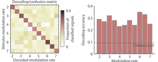
Subsequently, the circular distance (at each time point) between the single signal that was left out and the 11 templates is calculated, resulting in 11 circular distance time courses. This is followed by calculating the circular mean across time points for each of the 11 circular distance time courses. Finally, the decoded label of that signal is selected as the label of the template to which the mean distance is smallest.
The procedure (template calculation, circular distance, etc.) is repeated for each signal of each condition. The proportion of classified signals is then calculated (i.e., how often was a 2-Hz signal classified as 2-Hz signal, 2.5-Hz signal, etc.) resulting in a decoding/confusion matrix of which the diagonal reflects the decoding accuracy. The decoding/confusion matrix and the decoding or classification accuracy for each modulation rate are plotted above.
The simulated data and analyses were done using this simulation script. A function calculating the decoding/confusion matrix can be found here (under GNU license; self-check for errors; no warranty). Previous studies making use of this or similar analyses are Herrmann et al. (2013), Ng et al. (2013), and Luo & Poeppel (2007).